A practical guide to LLM inference optimization
Lugman Hussain Khan
LLM inference performance is shaped by more than the GPU or the model in isolation. The same model on the same hardware can behave very differently depending on how many requests arrive at once, how long the prompts are, how the weights are represented, and how the inference framework schedules the work.
An interactive assistant may care most about how quickly the first token appears. A RAG service may spend much more time processing input context. A batch workload may be willing to trade latency for higher throughput.
In this article, we use Qwen3–4B on an NVIDIA L40S to look at those trade-offs. We will look at how concurrency, context length, quantization, framework choice, and GPU capacity interact, and how to tune them around what the application actually needs.
Inference starts with the memory budget
The first constraint is VRAM. Qwen3–4B has roughly 4 billion parameters. In BF16, its weights require around 8 GB of memory. But model weights are not the only thing occupying the GPU.
The inference engine also needs memory for runtime operations and for the KV cache, which stores information from previously processed tokens so the model does not have to recompute them during generation.
The longer the context and the more requests being processed simultaneously, the larger that KV cache becomes. So the practical requirement is:
Model weights + KV cache + runtime overhead must fit inside GPU memory.
This gives us the basic memory requirement. Once the model fits comfortably, memory stops being the whole story.
Model fit does not define GPU performance
A 4B model can fit on both an NVIDIA L4 and an L40S, but fitting the model only answers the memory question. The L40S has 48 GB of VRAM compared with 24 GB on the L4, along with more memory bandwidth and compute capacity. That gives it a higher performance ceiling and more room for KV cache, longer contexts, and concurrent users.
Those specifications do not translate into a fixed speedup. The actual gain depends on how the GPU is being used, especially the amount of concurrency, context length, model precision, and the inference framework.
That is why the more useful comparison is not whether a GPU can run the model, but how throughput and latency behave under the workload you actually plan to serve.
Concurrency trades latency for throughput
Imagine serving a single user on an L40S. The request gets most of the GPU to itself, so latency is low. The problem is that a large part of the GPU’s total capacity is sitting unused.
Now start sending several requests at the same time. The inference engine can batch work together and use the GPU more efficiently. Total throughput rises significantly because the hardware is now doing more useful work in parallel.
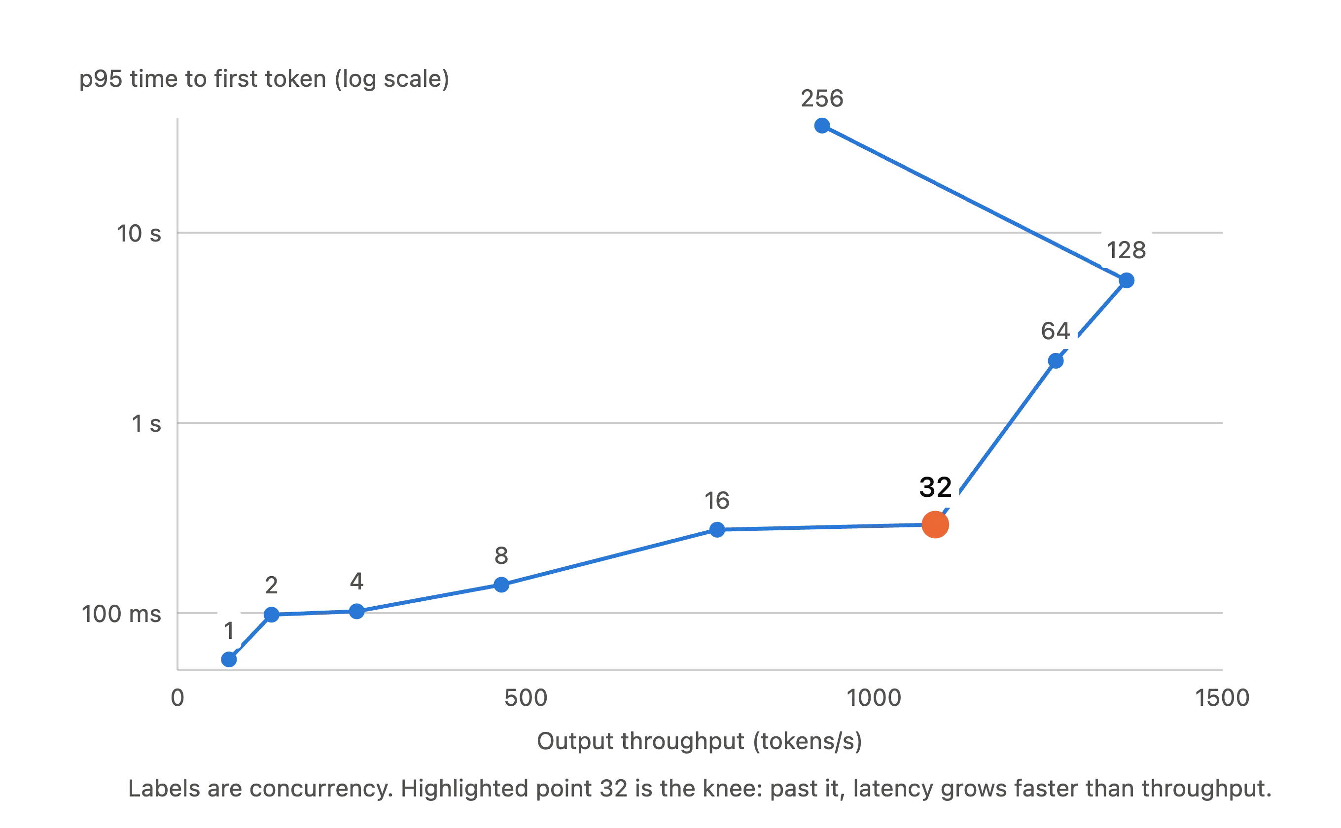
With Qwen3–4B in BF16 using vLLM, increasing concurrency from 1 to 32 raised output throughput from roughly 74 tokens per second to 1,088 tokens per second.
That is a very large improvement in GPU utilization. Latency increased as well, but initially the increase was manageable. At concurrency 32, p95 time to first token was still around 292 ms.
This is where we need to distinguish between a few latency metrics.
-
Time to First Token, or TTFT, measures how long the user waits before the response starts.
-
Inter-Token Latency, or ITL, measures how quickly new tokens arrive once generation has begun.
-
End-to-End latency measures how long it takes to finish the full request.
Each one describes a different part of the user experience.
For interactive applications, TTFT has a large impact on how responsive the system feels. ITL determines how smoothly the answer streams. End-to-end latency matters when the user needs the complete response before moving forward.
As concurrency moves from 32 to 64, something important starts to happen. Throughput increases from around 1,088 to 1,261 output tokens per second, which is only about a 16 percent gain. But p95 TTFT jumps from about 292 ms to more than 2.1 seconds.
Push concurrency further and throughput continues to improve for a while, but latency deteriorates much more quickly. For this particular Qwen3–4B workload, concurrency around 32 looks like a practical balance.
That does not mean 32 is the right number for every application.
A real-time assistant may prefer lower concurrency because fast response starts matter more. A batch-processing system may tolerate much higher latency if the goal is to maximize the total amount of work completed.
The important idea is to find the throughput and latency knee for your workload. That is much more useful than asking for the maximum tokens per second a GPU can produce.
Context length changes the latency profile
So far, we have been looking at relatively short prompts of around 1,000 tokens. That represents only one type of application.
A conversational assistant may regularly work with short prompts. A RAG system may insert several pages of retrieved information. A summarization or document-processing workload can easily reach tens of thousands of tokens.
Before the model starts generating an answer, it first has to process the complete input prompt. This stage is called prefill.
The longer the prompt, the more work the GPU has to complete before the first output token appears. That is why context length has a strong relationship with TTFT.
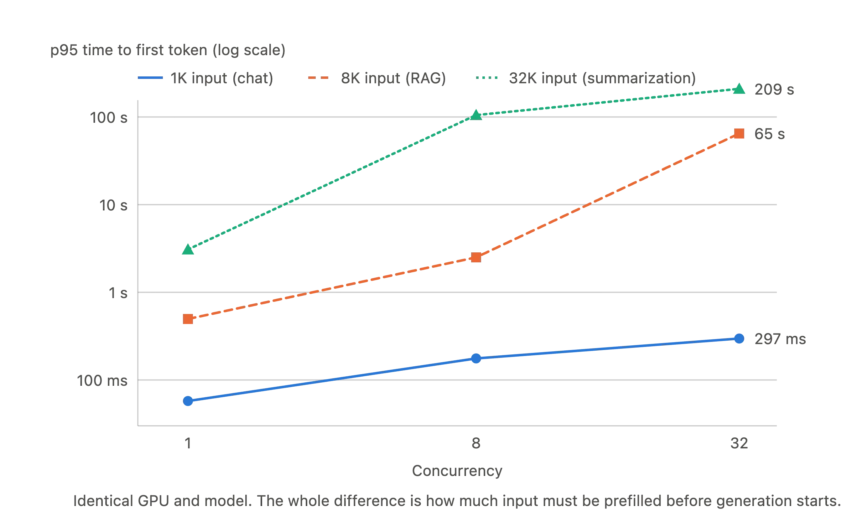
With one active request, a roughly 1K-token prompt had a median TTFT of around 56 ms. At 8K input tokens, that increased to roughly 487 ms. At 32K input tokens, it reached around 3.06 seconds.
The GPU and model are exactly the same in all three cases. The difference comes from how much input has to be processed before generation starts. The effect becomes much larger when long context and concurrency are combined.
At concurrency 8, p95 TTFT for the 1K workload stayed around 176 ms. The 8K workload reached roughly 2.5 seconds. With a 32K input, p95 TTFT crossed 100 seconds.
At that point, several long prompts are now competing for compute during prefill while also consuming significantly more KV cache. This explains why a benchmark using short prompts can badly overestimate the practical capacity of a RAG or document-processing system.
Quantization changes both capacity and speed
Once the basic workload is understood, there are several ways to improve efficiency before moving to larger hardware. One of the most common is reducing the precision of the model weights.
A BF16 model stores each parameter using 16 bits, while quantization techniques such as FP8 and AWQ represent weights using fewer bits. For this Qwen3–4B setup, that changes the model weight footprint substantially:
| Precision | Model weight size |
|---|---|
| BF16 | 8.06 GB |
| FP8 | 5.20 GB |
| AWQ | 2.68 GB |
Smaller weights leave more VRAM available for KV cache and reduce the amount of weight data that has to move through the GPU. When the hardware and inference engine support the format well, that can improve both capacity and inference speed.
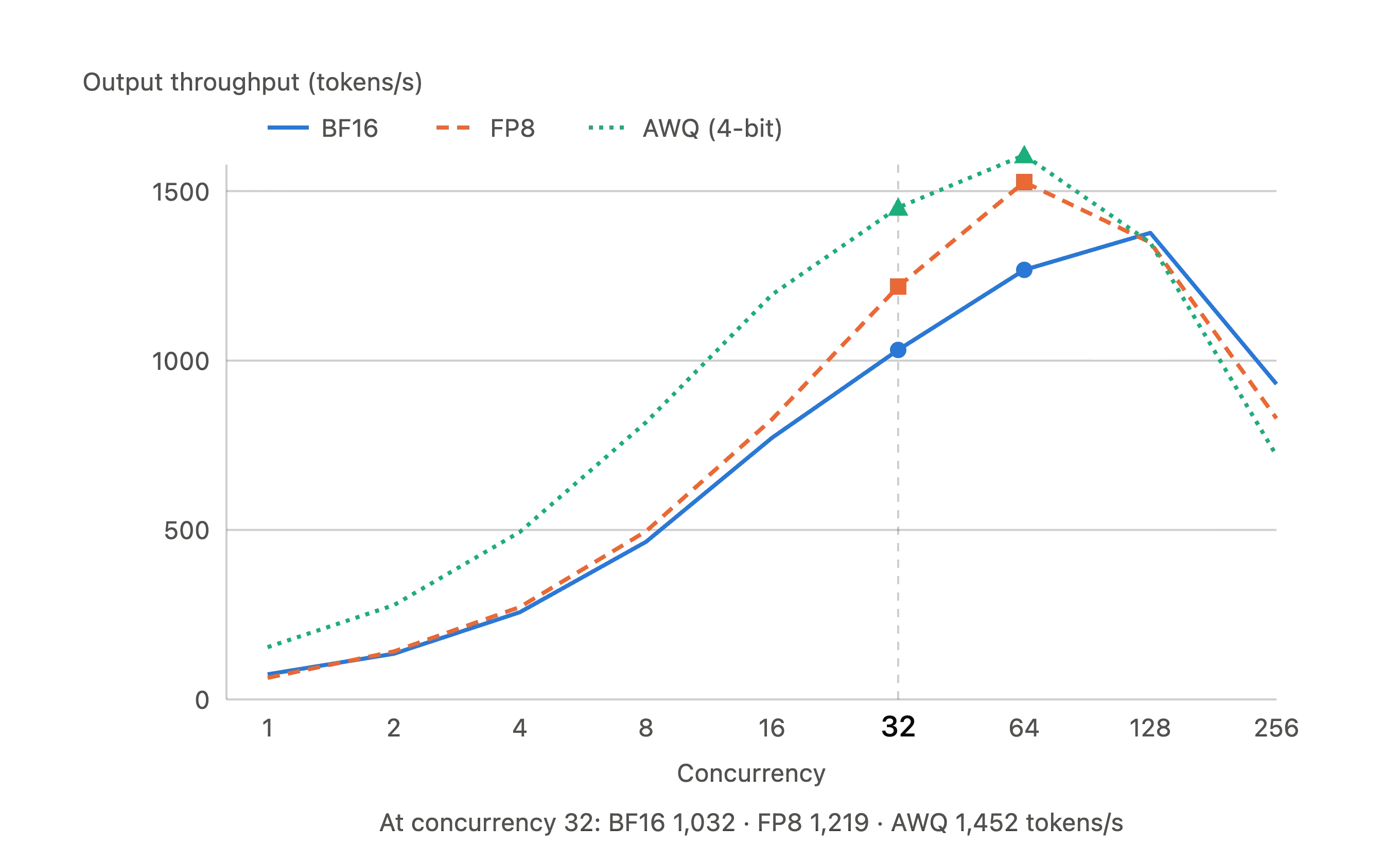
At concurrency 32, the difference was clear:
| Precision | Output throughput | p95 ITL | p95 end-to-end latency |
|---|---|---|---|
| BF16 | 1,032 tokens/s | 28.4 ms | 7.4 s |
| FP8 | 1,219 tokens/s | 25.6 ms | 6.7 s |
| AWQ | 1,452 tokens/s | 20.8 ms | 5.5 s |
FP8 improved throughput by about 18 percent over BF16, while AWQ was about 41 percent higher in this particular test and also had the lowest generation latency.
The important part is that the advantage was not identical at every load level. At very low concurrency, FP8 did not outperform BF16 in the same way, so the useful result is how a quantization format behaves under the load you expect to serve.
There is also a quality trade-off to consider. Quantization changes how model weights are represented, so performance testing should always be accompanied by an evaluation of whether model output quality remains acceptable for the application.
Choosing the serving framework
The inference framework controls batching, scheduling, memory management, KV cache handling, and many of the kernels used during inference. We compared vLLM and SGLang using the same Qwen3–4B BF16 workload on the L40S.
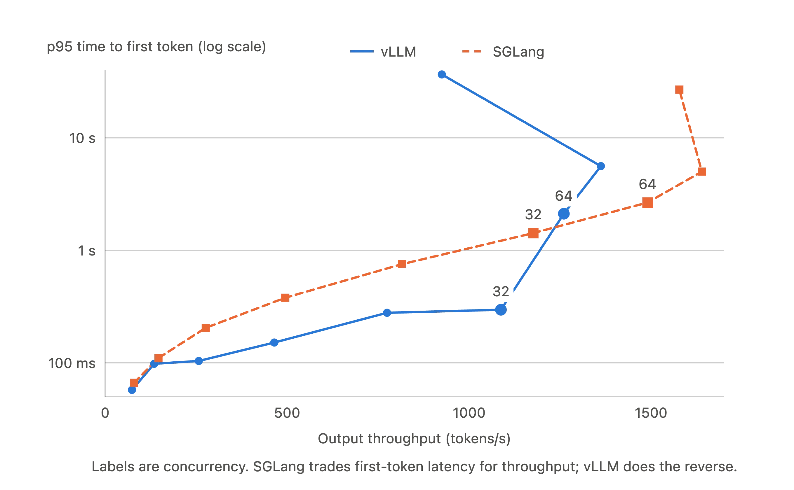
The trade-off becomes easier to see when the main results are put side by side:
| Concurrency | Framework | Output throughput | p95 TTFT | p95 end-to-end latency |
|---|---|---|---|---|
| 32 | vLLM | 1,088 tokens/s | 292 ms | 7.3 s |
| 32 | SGLang | 1,176 tokens/s | 1.39 s | 7.0 s |
| 64 | vLLM | 1,261 tokens/s | 2.12 s | 13.3 s |
| 64 | SGLang | 1,491 tokens/s | 2.66 s | 11.0 s |
SGLang delivered more throughput and slightly better generation and completion latency at these operating points, while vLLM returned the first token much sooner at concurrency 32. By concurrency 64, SGLang’s throughput advantage had grown further, but its TTFT was still higher.
So which one performed better depends on what the application values. An interactive assistant may prefer vLLM when fast response starts matter more, while a throughput-oriented workload may benefit more from SGLang.
Note: This result is specific to this model, GPU, and workload, so changing the model architecture, context distribution, quantization format, or hardware can change the comparison.
When to add capacity
After tuning concurrency, evaluating context behaviour, testing quantization, and comparing serving frameworks, you eventually reach the limits of the current hardware. That is when moving to a larger GPU becomes meaningful.
For example, if the highest throughput you can achieve while staying inside your latency target still cannot handle expected production traffic, then the workload needs more capacity.
That capacity could come from a faster GPU, additional GPUs, or more replicas. A GPU with more VRAM may also be necessary when the workload depends heavily on long contexts or high concurrency because KV cache capacity becomes a constraint. But once the hardware changes, the benchmarks need to be repeated.
Optimization does not stop here
Model precision and framework choice are not the end of the optimization space. Techniques such as Speculative decoding try to reduce the sequential cost of autoregressive generation by proposing multiple tokens and verifying them instead of advancing strictly one token at a time.
Newer approaches such as DSpark continue to explore this under concurrent serving workloads. They can improve decoding performance, but the same rule applies here. A published speedup is not your production speedup. What matters is the result with your model, hardware, traffic pattern, and latency target.
Takeaways
Start with the model. Determine how much VRAM its weights require and leave enough capacity for KV cache and runtime overhead.
Then define the workload. Understand how long your prompts are, how much output you expect, and how many users need to be served simultaneously.
Once the workload is clear, establish the latency targets that matter for the application. Then benchmark concurrency and find the point where adding more requests stops giving meaningful throughput improvements and starts producing disproportionate latency.
Evaluate the inference framework as well. The fastest framework on one GPU or model may not be the fastest everywhere else.
If performance is still limited by hardware, upgrade to a stronger GPU or distribute the workload across multiple units. Subsequent re-evaluation is necessary, as the new infrastructure will alter your optimal operating parameters.